Questions are subdivided by question type, which can be either Training or Forecast. Questions are also subdivided by distribution type, which can be either Discrete or Continuous. The four types of questions are thus discrete training, continuous training, discrete forecast, and continuous forecast.

Training questions are questions about facts and events for which the correct answers are known, but likely unknown by most users and therefore uncertain.

The primary advantage of training questions is that, because the correct answers are known, users can obtain instant feedback on their ability to assess uncertainty. The primary disadvantage is that it is possible to cheat on training questions because the correct answers are typically readily available on the internet. Users must of course resist the temptation to look up the correct answers when answering training questions, because this negates the benefit of answering training questions.

Forecast questions are questions about events that will occur in the future, to which the answers are unknown and thus uncertain.

The primary advantage of forecast questions is that the correct answers are in the future and therefore truly unknown; thus, it is impossible to cheat, intentionally or inadvertently. For this reason, forecast questions will provide the best measure of one’s ability to assess uncertainty reliably. Forecast questions are also of value because a common application of uncertainty assessment is to making decisions in the face of an unknown future. The primary disadvantage of forecast questions is that it takes time before the correct answers are learned. Thus, you do not get the immediate feedback on biases that you get from training questions.

A discrete question is a question (or event) for which there are a finite, and typically small, number of possible answers (or outcomes). Examples are true-false and multiple-choice questions. The possible answers to a discrete question are mutually exclusive (only one can be correct) and exhaustive (the probabilities of all the possible answers must sum to 100%). An example discrete training question is “Iron is denser than gold; True or False?”

A continuous question is a question (or event) for which the answer (or outcome) is always a numerical quantity. Furthermore, there are a large, and commonly infinite, number of possible values of the answer. For example, the answer to the continuous training question of the driving distance in miles between Houston and Denver can technically always be measured with more accuracy: 1034, or 1034.2, or 1034.237, etc. Thus, there are an infinite number of possible values. The question of the year the first European printing press was invented, while technically a discrete question, has so many possible answers that it would be impractical to ask it as a discrete question. It is effectively a continuous question and, thus, is treated as a continuous question in FixMyBias.

Upon opening the application, you will land on the Forecast Questions page. To answer training questions, navigate to the Training Questions page. By default, all forecast and training questions available for answering are displayed on these two pages, respectively. Questions can be further filtered by question text, Question Status (All, Available or Unavailable), Distribution Type (All, Discrete or Continuous), Tags (All, Science, Sports, etc.), and, for training questions, by Sets (All, Not part of set, Set 1, Set 2, etc.). A set is a group of questions (typically 10 or 20) that might have a common source or common theme.

If multiple filters are applied, a Boolean AND operation is applied. For example, selecting the Distribution Type Discrete and selecting the Tag Sports will result in a set of questions that are discrete AND have a tag of Sports. Thus, each application of a filter will either reduce the number of questions displayed or leave the number of questions the same (if there are no questions to which the filter applies).

Filtering on Available (the default) under Question Status displays questions that are available for assessment, which for training questions means those that have not yet been answered and for forecast questions means those that have not yet closed (the correct answer is not yet known). Filtering on Unavailable displays questions that are unavailable for assessment, which for training questions means those that you have already answered and for forecast questions means those that have closed (the correct answer is known).

The number in parentheses at the top of the questions pages indicates the number of questions displayed on the page according to the current filter selections.

Once you have a filtered subset of questions displayed on either the forecast or training questions page that you would like to answer, you can begin answering questions by clicking on the text of any question on the questions page. This will take you to the question-answer page, where you can enter answers to the question displayed and then hit Submit to submit your answers. The next (“>”)and previous (“<”) buttons will take you through the filtered subset of questions that were displayed on the questions page. You can answer questions that you want to answer and skip questions that you do not want to answer. When you are finished, you can select “Return to Forecast/Training questions list.”

A training question can be answered only once, because the correct answer is displayed to the user immediately after probabilistic answers to the question are submitted.

A forecast question can be answered as many times as desired until the correct answer is known and the question is closed. However, the question can be answered no more than once per day. Typically, the close date is known and displayed ahead of time, but this is not always firm (e.g., for a forecast of the baseball World Series, which can take as few as four games and as many as seven games to be resolved). One might consider making multiple probabilistic assessments over time for the same forecast question because the available information related to the future question may change over time, which means one’s uncertainty related to the question may change as well.

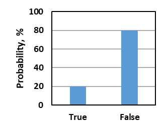
To answer a discrete question, you assign probabilities to all the possible choices such that the probabilities sum to 100%. You should assign probabilities that correspond to your relative certainty about the different choices. For example, if you are reasonably, but not completely, sure the correct answer to the discrete training question “Iron is denser than gold; True or False?” is False, you might assign 20% probability to True and 80% probability to False (figure below). If you are completely unsure, i.e., you have absolutely no knowledge about the choices, then you should assign equal probabilities—50% to each choice for a true-false question and 25% to each choice for a 4-choice multiple-choice question. When you are satisfied with your probability selections, hit the green Submit button to submit your answers.

To save time, hitting the Auto Fill button will divide the remaining probability evenly among the blank probability fields. For example, for a true-false question, if you enter 70% in one cell and hit the Auto Fill button, it will put 30% in the blank cell. For a 4-choice multiple-choice question, if you were reasonably sure about one choice but equally unsure about the other choices, you could enter 70% in the one cell you are sure about, hit the Auto Fill button, and it will assign 10% to each of the remaining 3 blank cells. The Clear Answers button will clear the probabilities for all possible answers so you can start over.

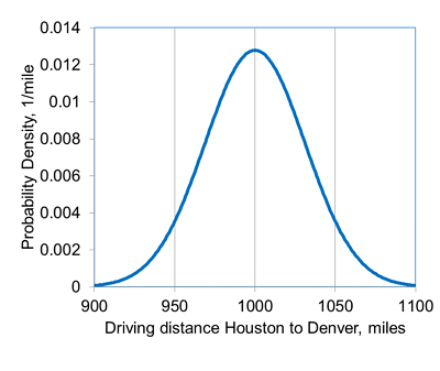
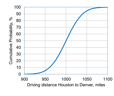
You express your uncertainty about the answer to a continuous question by assigning numerical values corresponding to different values of cumulative probability (i.e., by specifying points on a cumulative distribution function, or CDF). By default, the cumulative probabilities to which you assign numerical values are 10%, 50% and 90%. To 10% cumulative probability, you should first assign a low estimate for the uncertain quantity (aka the P10 value, where “P” stands for percentile) such that there is only a 1 in 10 chance that the correct value is less than your P10 value. To 50% cumulative probability, you should assign a middle value (the P50) such that it is just as likely the correct value is less than the P50 value than it is greater than the P50. To 90% cumulative probability, you should first assign a high estimate for the uncertain quantity (the P90) such that there is only a 1 in 10 chance that the correct value is greater than your P90 value. For example, an answer to the continuous training question of the driving distance in miles between Houston and Denver might be expressed by the probability density function (PDF) and corresponding cumulative distribution function (CDF) below, which have a P10, P50 and P90 of 960, 1000 and 1040 miles, respectively.

You can change cumulative probabilities to which you assign numerical values if you choose. You can also add and delete rows in order to specify as many or as few points on the distribution as you want. If you prefer, you can answer the question by specifying points on a decumulative probability distribution instead of a cumulative distribution. In this case, you would assign a high numerical value to 10% cumulative probability and a low numerical value to 90% cumulative probability. The order of the numerical values or the cumulative probabilities does not matter. However, the numerical values must either increase monotonically with increasing cumulative probability or decrease monotonically with increasing cumulative probability. If they do not, the system will flag this as an error and it must be corrected before your answers can be submitted.

You cannot see the correct answer to a training question until you submit answers to the question. After submitting, you will immediately see the correct answer displayed below your answers. After you leave the question-answer page, if you later want to come back to a question to see your answers and the correct answer, you will have to select the All or Unavailable Question-Status filter on the Training Questions page (because the question is no longer available for answering) and then open the training question of interest.

If you want to see your previous answers to a forecast question that has not yet closed, you can open the question at any time (with the All or Available Question-Status filter selected) from the Forecast Questions page and you will see the last answers you submitted for this question. We will soon be adding a plot that will show all of your previously submitted answers to the question. You cannot see the correct answer until the question has closed. For a forecast question that has closed, you will first have to select the All or Unavailable Question-Status filter on the Forecast Questions page (because the question is no longer available for answering) and then open the forecast question of interest to see the correct answer and your previously submitted answers.

Click on Scoring in the menu at the top of the page. There will you see a collection of plots and tables summarizing your biases and your estimation/prediction reliability.

A variety of options are available for filtering assessments for scoring. Assessments can be filtered by question text, Question Type (All, Forecast or Training), Distribution Type (All, Discrete or Continuous), Assessment Date Range, Tags (All, Science, Sports, etc.), and Sets (All, Not part of a set, Set 1, Set 2, etc.). A set is a group of questions (typically 10 or 20) that might have a common source or common theme.

If multiple filters are applied, a Boolean AND operation is applied. For example, selecting the Question Type Forecast and selecting the Tag Sports will result in a set of assessments that are forecasts AND have a tag of Sports. Thus, each application of a filter will either reduce the number of assessments scored or leave the number of assessments the same (if there are no assessments to which the filter applies).

The primary emphasis in FixMyBias is measuring the reliability, or calibration, of probabilistic assessments. That is, when 90% probability is assigned to possible answers to questions, are those answers correct about 90% of the time, and likewise for all other probability assignments? If they are not, then this indicates the presence of biases in assessment.

Of secondary importance is the accuracy, or resolution, of probabilistic assessments. For discrete assessments, more accurate assessments are those to which high probabilities are assigned to correct possible answers to questions. For continuous assessments, more accurate assessments are those to which small probability ranges are assigned around the correct answers to questions.

One of the keys to making good decisions under uncertainty is assigning well-calibrated probabilities to the possible outcomes associated with the decisions. The presence of biases, such as overconfidence and optimism, can result in poor decisions and suboptimal consequences (Kahneman 2011). Good decisions can be made regardless of how little or how much information one has about the event or topic under consideration, provided the probability assessments are reliable (i.e., well calibrated).

Granted, there may be more value associated with a particular decision if more information can be acquired and thus more accurate probability assessments can be made. However, there will be a cost associated with acquiring additional information (e.g., time spent on research or cost associated with acquiring new information), and the question is then whether the value of the information is greater than the cost. This is a value-of-information problem and is beyond the scope of this application.

Calibration is measured by comparing probabilistic assessments to the correct answers for questions answered. Probabilistic calibration can be measured only with a group of probabilistic assessments. To start, we collect all the assessments with a particular probability assigned, say 90%. For example, you might have assigned 90% probability that the second answer to Question 35 is correct, 90% probability that the third answer to Question 56 is correct, and so on. Then, we calculate the percentage of answers to which you assigned 90% probability that were actually correct (we call this the Proportion Correct). Let’s say that the proportion correct was 70% for assessments to which you assigned 90% probability. We then repeat this procedure for all probabilities that were assigned to particular assessments, e.g., 75%, 50%, 25%, 10%, and so on. Calibration is measured by comparing proportion correct to Probability Assigned for all values of probability assigned—in tabular form, in graphical form, and in the calculated calibration score. The closer the proportion correct values are to the probability assigned values, the greater the reliability of the probabilistic assessments.

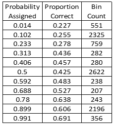
The calibration table is the collection of Proportion Correct versus Probability Assigned values for all probabilistic assessments included in the scoring. The calibration table also lists the number of assessments for each probability assigned (the Bin Count).

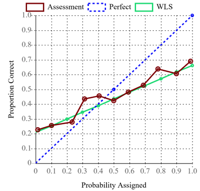
The calibration plot displays a plot of the Proportion Correct versus Probability Assigned values listed in the calibration table. This is the raw calibration curve (maroon). The calibration plot also displays the straight line (green) that best fits the raw calibration curve. The best-fit line is found using weighted least-squares regression, where each (probability assigned, proportion correct) point is weighted by the number of assessments for the probability assigned. This best-fit straight line is used in interpretation. The calibration plot also displays the unit-slope line (blue dashed) that corresponds to perfect calibration.

So that both discrete and continuous questions can be assessed in the same calibration table and calibration plot, each answered discrete and continuous question is ultimately reduced to a set of distinct probabilistic assessments. For example, the answers to the two-choice discrete question “Which city is the capital of Texas, Austin or Houston?” might result in the following two probabilistic assessments: correct answer = Austin with probability 75%, and correct answer = Houston with probability 25%. Comparing to the known correct answer (Austin), the first assessment would be correct and the second would be incorrect for the purpose of calculating proportion correct. The answers to continuous question “In what year did Texas become a U.S. state?” might result in the following three probabilistic assessments: correct answer ≤ 1820 with probability 10%, correct answer ≤ 1840 with probability 50%, and correct answer ≤ 1860 with probability 90%. Because the known correct answer is 1845, the first two assessments would be incorrect and the third assessment would be correct for the purpose of calculating proportion correct.

For consistent interpretation of directional bias, all continuous assessments made using the decumulative probability distribution convention (where the P90 is a low estimate and the P10 is a high estimate) are converted to the cumulative probability distribution convention (where the P10 is a low estimate and the P90 is a high estimate) for the purpose of calculating probability assigned and proportion correct.

Because users are free to assign whatever probabilities they choose, and because proportion correct is a statistical quantity requiring multiple assessments, it would be impractical to calculate a proportion correct for every single probability value assessed by a user. Thus, assessments are grouped into bins (currently 11) by probability assigned for the purpose of calculating probability assigned and proportion correct. For example, the first bin contains all assessments with probabilities assigned that fall between 0 and 0.0909 (1/11). For each bin, the average probability assigned is calculated for all the assessments in the bin; this value becomes the probability assigned in the first column of the calibration table and the x-axis value of the raw calibration curve on the calibration plot. The proportion correct in each bin is calculated by dividing the number of correct assessments (determined by comparing to the known correct answer to each question, as discussed above) by the total number of assessments in the bin (bin count). This value becomes the proportion correct in the second column of the calibration table and the y-axis value of the raw calibration curve on the calibration plot.

To be perfectly calibrated, or perfectly reliable, means that your beliefs and probability assessments are perfectly aligned with reality, on average. It means that when you assess probabilities of 90%, you will be correct 90% of the time, on average, and likewise for all other probability assessments. To be perfectly calibrated means that you are unbiased in your probability assessments.

Biases are distortions in reasoning and judgments that result in probability assessments that are not perfectly calibrated. Subjective probability assessments are a function of both evidence (information) available and biases. Biases are the part of probability assessments that are not based on evidence.

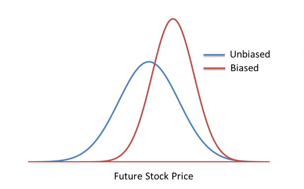
Researchers have identified over 100 different cognitive biases that affect estimation and prediction. It is impossible to distinguish between these different biases individually by calibrating probabilistic assessments. However, some have observed that, for continuous assessments, all these biases can be boiled down to two principal biases—confidence bias and directional bias (McVay and Dossary 2014, Alarfaj and McVay 2020). Confidence bias relates to the uncertainty of the estimate, i.e., the width of the distribution. Directional bias relates to the central value of the estimate, i.e., the directional shift of the distribution. The following figure shows an unbiased continuous probability distribution of future stock price (blue) and a biased distribution of the same stock price (red) that is both overconfident (is too narrow and thus underestimates uncertainty) and positively biased (is shifted to the right). If one has a personal stake in the estimate (e.g., if one owns this stock), then this positive directional bias could be considered optimism bias.

It has been demonstrated by many researchers over decades that overconfidence (underestimation of uncertainty) is very common, likely the most common bias. Some call overconfidence the primary bias, the gateway bias, or the mother of all biases (Moore 2020). Other biases are secondary—it is the presence of overconfidence that permits other biases, like directional bias, to exist. Consequently, the detection and elimination of overconfidence can be helpful in mitigating other biases as well.

Overconfidence is very common in discrete probabilistic assessments as well. Directional bias can also be present in some contexts. For example, in estimates and predictions in politics and government policy, if overconfidence is present there can also be directional bias towards progressivism or conservatism. However, because discrete probabilistic assessments are often nonquantitative, it is more difficult to separate confidence and directional biases than it is for continuous assessments, which are always quantitative. For this reason, and because overconfidence is the gateway bias, we generally focus on just overconfidence bias for discrete assessments, trusting that mitigation of overconfidence will mitigate other biases as well.

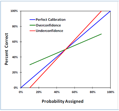
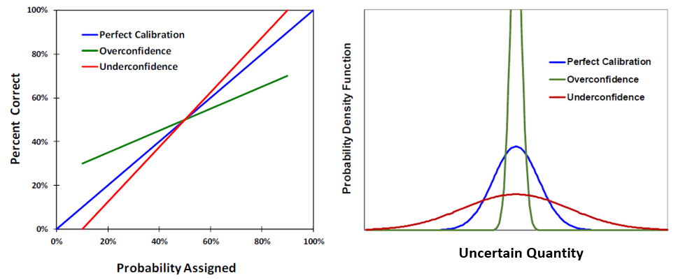
Confidence bias is indicated by the slope of the calibration curve on a calibration plot. The following figure shows three different calibration curves. A curve that falls on the unit-slope line is perfect calibration (blue curve). Overconfidence (underestimation of uncertainty) is indicated by a calibration curve with slope less than one (green curve). Underconfidence (overestimation of uncertainty) is not common, but when present is indicated a slope greater than one (red curve).

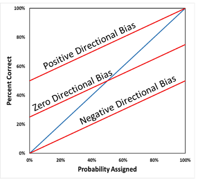
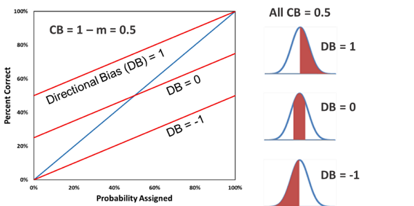
For continuous assessments, directional bias is indicated by the vertical shift in the calibration curve. The following figure shows three different calibration curves (all red), all with moderate overconfidence (slope less than one). Positive directional bias is indicated by an upward shift in the calibration curve (top curve), while negative directional bias is indicated by a downward shift in the calibration curve (bottom curve). Zero directional bias is indicated by a calibration curve that goes through the (50%,50%) point on the plot. For consistent interpretation of directional bias, in this application all continuous assessments made using the decumulative probability distribution convention (where the P90 is a low estimate and the P10 is a high estimate) are converted to the cumulative probability distribution convention (where the P10 is a low estimate and the P90 is a high estimate) in constructing the calibration plot.

Caution must be exercised in interpreting a calibration plot that has a mix of continuous and discrete assessments, as in the following figure. The first thing to notice is that the raw calibration curve (maroon) is somewhat noisy. This is because the curve contains a mix of continuous and discrete assessments, and there are large differences in the number of assessments in the bins, shown in the corresponding table. Because of the noise, it is best to base the interpretation on the weighted-least-squares best-fit straight line (green), which indicates overconfidence (slope less than one) and negative directional bias (slight downward shift). With due caution, the most likely interpretation is that there is overconfidence in the discrete assessments, and overconfidence and slight negative directional bias in the continuous assessments. This could be investigated further by filtering to generate separate calibration plots for the continuous assessments and discrete assessments.

The table at the top of the Scoring page shows calculated scoring metrics. The first two columns show the Brier score and the calibration score (which is one component of the Brier score). The last four columns show the slope and intercept of the least-squares regression line on the calibration plot and values of confidence and directional biases calculated from this line. Strictly speaking, calculation of directional bias applies to only continuous assessments. Thus, interpretation of directional bias is unclear for a set of assessments that contains any discrete assessments. Also, the Brier score is typically used for scoring discrete assessments and has limited applicability to continuous assessments (e.g., it cannot be driven to zero even for a set of perfect continuous assessments). Thus, interpretation of Brier score is unclear for a set of assessments that contains any continuous assessments. For a set of assessments that includes both discrete and continuous assessments, only calibration score (measure of average distance of the calibration curve from the unit-slope line), WLS slope and confidence bias have any meaningful interpretation.

The calibration score, also known as the reliability score, is the most important metric. It measures the correspondence between the probabilities assigned and the proportions of correct assessments, i.e., how well assessed probabilities match reality. On a calibration plot, the calibration score measures the average squared distance of the raw calibration curve from the unit-slope line. Thus, it measures the deviation from perfect calibration. A lower calibration score is better, and a calibration score of zero corresponds to perfect calibration. The calibration score applies to both continuous and discrete probability assessments.

The Brier score is a proper scoring rule that measures the overall quality of a set of probability assessments. It applies to discrete assessments only. A lower Brier score is better, and zero is a perfect score. The Brier score includes calibration score as one of its components. Thus, it considers how well assessed probabilities match the frequency of correct outcomes. However, it also includes a resolution score, which considers the sharpness, or boldness, of the discrete assessments. In other words, resolution measures how close the assigned probabilities are to zero and one. Consider a set of discrete, binary, true-false questions in which the correct answers are True in half of the questions and False in half of the questions (base rate of 0.5). An assessor could assign true-false probabilities of 50%-50% to every question and be perfectly calibrated. However, this would not be a particularly useful set of assessments, and the Brier score includes a penalty for the low resolution. A more useful, and accurate, set of assessments would have high probabilities assigned to the correct answers and low probabilities assigned to the incorrect answers. The lowest possible Brier score is zero, when the assessor always assigns a probability of one to the correct answers, while the highest possible score is two, when the assessor always assigns a probability of zero to the correct answers.

For ease in interpretation of the calibration plot (because it is sometimes not smooth), and for calculation of confidence and directional biases, we calculate the straight line (green) that best fits the raw calibration curve (maroon). This is done using weighted least-squares (WLS) regression, where each data point on the raw calibration curve is weighted by the number of assessments constituting the data point (bin count in the calibration table). Large differences in numbers of assessments can result in a WLS straight line that visually does not appear to fit the raw calibration curve, even though it is the best fit considering all the data points. WLS slope is the slope of this best-fit straight line, while WLS intercept is the y-intercept of the best-fit straight line.

WLS slope can also be thought of as a Normalized-Proportion-Correct Range for continuous assessments. For example, on a calibration curve, if your P10s correspond to a proportion correct of 30% and your P90s correspond to a proportion correct of 70%, then your 80% (90% – 10%) probability range corresponds to only a 40% (70% – 30%) proportion-correct range. The slope of this calibration curve, and thus the normalized-proportion-correct range, is 0.5, the ratio of 40% to 80%. Thus, the WLS slope indicates the fraction of the probability range the proportion-correct range will be for any probability range (e.g., the proportion-correct range for a P5-P95 probability range would be 45%).

Confidence bias (CB) is a quantitative measure that indicates both the direction and degree of confidence bias (underestimation or overestimation of uncertainty). CB is calculated from WLS slope, the slope of the weighted-least-squares straight-line fit of the raw calibration curve. Like the calibration and Brier scores, CB is defined so that a value of zero is ideal. Confidence bias ranges from -1 (complete underconfidence) through 0 (unbiased) to 1 (complete overconfidence, or a point estimate). Additional details on the model for calculating confidence bias and directional bias can be found in McVay and Dossary (2014) and Alarfaj and McVay (2020).

For overconfidence, CB is simply 1 – WLS Slope (there is a different equation for underconfidence, which is not very common). In the left figure below, the green calibration curve has CB = 0.5, the blue curve has CB = 0, and the red curve has CB = -0.2. All of these calibration curves have zero directional bias. If the assessments are all continuous, the right figure below shows what the corresponding probability distributions would be, on average, for each calibration curve, assuming the blue distribution is the true, unbiased distribution.

Directional bias (DB) is a quantitative measure that, for continuous probability assessments, indicates both the direction and degree of the shift of the estimated distribution relative to an unbiased distribution. DB is calculated from both WLS slope and WLS intercept, the slope and intercept, respectively, of the weighted-least-squares straight-line fit of the raw calibration curve. DB is also defined so that a value of zero is ideal. DB ranges from -1 (complete negative directional bias) through 0 (unbiased directionally) to 1 (complete positive directional bias). If the assessor has a personal stake in a value-based assessment (e.g., estimation of the future price of a stock which the assessor owns), then positive DB would be optimism bias and negative DB would be pessimism bias. If the assessor has a personal stake in a cost-based assessment (e.g., estimation of the cost to repair a car which the assessor owns), then negative DB would be optimism bias and positive DB would be pessimism bias. Additional details on the model for calculating confidence bias and directional bias can be found in McVay and Dossary (2014) and Alarfaj and McVay (2020).

For consistent interpretation of directional bias, all continuous assessments made using the decumulative probability distribution convention (where the P90 is a low estimate and the P10 is a high estimate) are converted to the cumulative probability distribution convention (where the P10 is a low estimate and the P90 is a high estimate) in constructing the calibration plot and calculating DB. In the left figure below (in which all three red calibration curves have CB = 0.5), the top curve corresponds to complete positive directional bias and has DB = 1. The middle curve has no directional bias and has DB = 0. The bottom curve corresponds to complete negative directional bias and DB = -1. To the right are corresponding average probability distributions for each calibration curve, assuming in each case the blue distribution is the true, unbiased distribution and red truncated distribution is the assessed, biased distribution.

In a public application like this where all users have access to all questions, it is difficult to ask questions that will allow individual users to measure directional bias consistently. Positive DB in one category of questions might cancel out negative DB in another category of questions. Measuring optimism-pessimism biases presents even more challenges, as optimism-pessimism biases are often transactional in nature. Optimism bias in the buyer in a potential transaction would correspond to pessimism bias in the seller in the transaction. All of this is to say that caution should be exercised in interpreting directional bias. Judicious use of question filtering may be required to obtain useful measures of directional bias for bias mitigation and decision making.

If you determine from previous assessments that you are not perfectly calibrated, you are most likely overconfident. This will be indicated by a slope less than one on the calibration plot, calibration and Brier scores greater than zero, and confidence bias greater than zero. While you might be biased in other ways (e.g., directionally), overconfidence is very likely the primary problem and should be the initial focus for improvement. By filtering on distribution type, you can determine if the overconfidence is primarily in discrete assessments or continuous assessments, or in both.

You can use the calibration plot of past assessments as a guide for correction of new assessments. For discrete assessments, suppose when you have assessed 90% probability (x-axis value) in the past you have been correct (y-axis value) only 70% of the time. Going forward, when your initial reaction is to assign 90% probability, assign 70% probability instead. Proceed likewise for other probability assignments.

For continuous assessments, if you are overconfident this means your distributions are too narrow—your P10s are not low enough and your P90s are not high enough (this might be a little more complicated if directional bias is present). Remember that all assessments are converted to a cumulative distribution convention (P10 low, P90 high) prior to scoring; adjust accordingly if you prefer to use a decumulative distribution convention (P90 low, P10 high). If your distributions have been too narrow in the past, then you will need to widen your distributions going forward. How much you should adjust for continuous assessments is not as obvious from the calibration plot as it is for discrete assessments. While there are analytical methods available for extrapolating the distribution (e.g., see Capen 1976), most people will learn how much adjustment is required with experimentation and repetition. Because overconfidence is the gateway bias, correcting overconfidence will usually go a long way in also correcting directional biases in continuous assessments.

For both discrete and continuous assessments, iteration will likely be required to obtain near-perfect calibration. This can be accomplished most quickly using training questions. Answer a set of training questions, check calibration of that question set, then adjust appropriately in answering a new set of training questions. Repeat until biases are eliminated. The best test of your probabilistic assessment ability, however, is forecasting into a truly unknown future. You can use the same iteration procedure with forecast questions, although this will obviously take more time due to the delays in learning the correct outcomes.

You can use the Assessment Date Range filter on the Scoring page to determine your probabilistic assessment performance over time. Generate and record scoring metrics for different time periods and then compare to see if calibration and Brier scores and confidence and directional biases are all decreasing over time. We will be soon adding a plot that displays all the relevant scoring metrics as a function of time to make this comparison easier.

Note that both a probabilistic assessment and the correct answer to a question are required for scoring, and that assessment date range filters on the day an assessment was made. Thus, scoring for a particular time period may not include all assessments made during the time period if some of the assessments were forecasts that were not resolved (the correct answers were not learned) during the time period. For example, suppose on February 1, 2026, scoring was checked for assessments made in the month of January 2026. Scoring of those same January 2026 assessments on March 1, 2026, could be different if some of the forecast questions answered in January closed and the correct answers were learned in February. This should be kept in mind as you compare your performance over time.

Business and life are full of uncertainty. Business and life decisions are made in the midst of uncertainty.

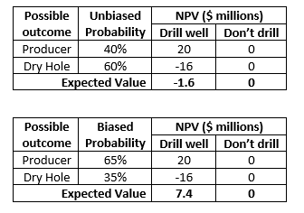
A decision consists of choices, uncertain outcomes and probabilities, and values (payoffs) associated with each combination of choice and uncertain outcome. A simple decision for drilling a well is shown in the following table. For simplicity in this example, the uncertain outcome of drilling the well is considered to have only two possibilities—producer vs dry hole.

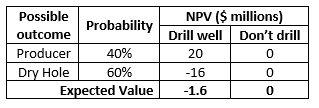
The uncertainty in well outcome in this example is expressed quantitatively in terms of probabilities. Assessing the uncertainty in possible outcomes is an important part of the decision-making process. Quantifying uncertainty allows the decision maker to assess the upside potential and downside potential (risk) associated with the decision in order to make a good decision. In this example, because there is a 60% chance (or risk) of drilling a dry hole with a large cost, the best decision is to not drill the well because the expected value (probability-weighted average) of drilling the well is less than the expected value of not drilling the well.

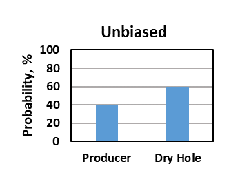
While uncertainty can be expressed with words, the best way to express uncertainty is quantitatively with probabilities. There are two fundamental types of probabilistic assessments: discrete and continuous. In the decision table below, the possible outcomes are expressed in terms of two discrete, exhaustive, mutually-exclusive outcomes. Exhaustive means these are the only two possible outcomes; thus, the probabilities must sum to 100%.

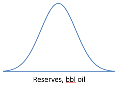
The outcome of the well could also be expressed in terms of reserves, in barrels of oil, in the form of a continuous probability distribution.

In general, humans are poor at assessing uncertainty, i.e., we are biased. We have an almost universal tendency for overconfidence, or underestimation of uncertainty. This is well documented in many studies (e.g., Tversky and Kahneman 1974, Capen 1976). We are more certain than we have a right to be. Humans also have a general tendency for optimism, i.e., to think that things will turn out better than they do on average (e.g., Weinstein 1980, Merrow 2012). The tendency for optimism is apparently not as strong or prevalent as the tendency for overconfidence; sometimes we are overconfident and pessimistic.

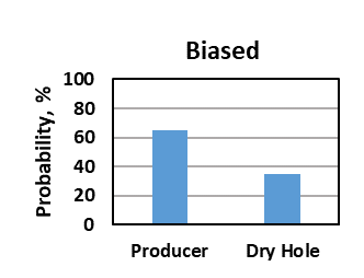
For discrete probabilistic assessments, overconfidence and optimism results in overestimation of the probability of a desirable outcome. In a well-drill decision, instead of an unbiased 40% probability of a producer, overconfidence and optimism biases might result in the analyst assigning a 65% probability of a producer (figure below).

For continuous probabilistic assessments, overconfidence bias results in distributions that are too narrow (red curves in figure below), while directional bias (e.g., optimism or pessimism) shifts the distribution directionally.

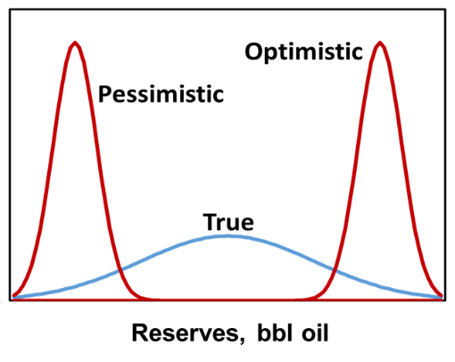
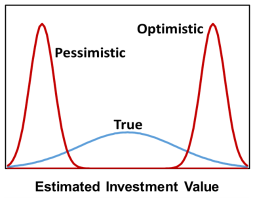
If we are making decisions with unreliable uncertainty assessments, we will sometimes, if not often, make poor decisions. In general, if we are overconfident and optimistic (figure below), we will invest in some investments that we should not invest in. Likewise, if we are overconfident and pessimistic (figure below), we will not invest in some investments that we should invest in, resulting in missed opportunities.

In a decision problem using discrete distributions, instead of an unbiased 40% probability of a producer, overconfidence and optimism biases might result in the analyst assigning a 65% probability of a producer, which could change the decision from not drilling the well (good decision) to drilling the well (poor decision).

The result of making poor decisions in business is reduced value. McVay and Dossary (2014) and Alarfaj and McVay (2020) demonstrated that persistent overconfidence and optimism in project selection can result in substantial disappointment in project-portfolio value. That is, the actual or realized portfolio value will be lower, on average, than the estimated portfolio value. They also demonstrated that persistent overconfidence and pessimism can result in realized portfolio values higher than estimated, but lower than they would be, on average, if these biases were not present. In portfolio selection, realized portfolio values are maximized when project evaluations are completely unbiased—neither overconfident nor underconfident, and neither optimistic nor pessimistic.

These conclusions are corroborated by petroleum industry performance. Many authors have reported that for decades the industry has underperformed due to chronic overconfidence and optimism in project evaluation (e.g., Capen 1976, Rose 2004, Brashear et al. 2001, Nandurdikar 2014). One key to optimizing decision making and value creation is eliminating biases in uncertainty assessment. It is safe to say that the same principles apply to decision making in all of life.

To eliminate biases, it is first necessary to measure them. The only way to measure biases is to make probabilistic assessments, or estimates, and then to compare the probabilistic assessments to the actual values when they become known.

If we are unbiased and are estimating uncertainty reliably, then outcomes will be consistent with the probabilities assigned. For example, with discrete assessments, if there are 100 wells for which we have estimated a 70% probability of being a “good” well, then about 70 of these wells should turn out to be “good” wells once they have been drilled and we know their performance. Continuous probabilistic assessments are often expressed in terms of cumulative probabilities. For example, a P10 means there is a 10% probability the actual value will be less than or equal to the P10 value (for the convention in which the P10 is the low number and the P90 is the high number). If our continuous probabilistic assessments are unbiased, or reliable, then the actual reserves values will be less than the P10 reserves estimates for about 10 wells out of 100 once the actual reserves are known.

The reliability of probabilistic assessments can be expressed on a calibration plot (figure below). A group of probabilistic assessments are unbiased, or perfectly reliable, if the calibration curve falls on the unit-slope line (blue). A slope less than 1 indicates overconfidence (green). For example, for a group of P90 assessments, the actual value was less than the P90 estimate only 70% of the time (the analyst was overconfident by estimating the actual value would be less than the P90 value 90% of the time rather than 70%). Underconfidence (overestimation of uncertainty) is indicated by a slope greater than 1 (red). However, underconfidence is rare.

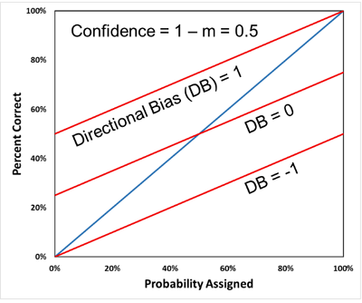
We can also measure directional, or optimism-pessimism, biases from the intercept of the calibration plot. In the figure below, we show that we can measure confidence and directional biases quantitatively. Confidence bias (CB) ranges from -1 (complete underconfidence) through 0 (unbiased) to 1 (complete overconfidence, or a point estimate). Directional bias (DB) ranges from -1 (complete negative directionally, which is pessimism for value-based assessments) through 0 (unbiased directionally) to 1 (complete positive directionally, which is optimism for value-based assessments). See McVay and Dossary (2014) and Alarfaj and McVay (2020) for more detail on these concepts.

Biases can be measured with two different kinds of probabilistic assessments. Training questions, for which the answers are known but unknown to the user, can be asked about virtually any subject, such as science, literature, history, sport, and technology. Some may question the value of questions in other subjects if their primary interest is improving their ability to assess uncertainty in a particular subject area, such as weather or oil production forecasts. However, studies show that experts can be just as poor at assessing uncertainty as novices (Lichtenstein and Fischhoff 1977), which indicates that assessing uncertainty is a different skill than petroleum engineering, astrophysics or any other subject. Thus, training that improves one’s ability to assess uncertainty generally will benefit analysts in their subjects of expertise, vocation or interest (although the benefits may not be the same in all subjects).

Biases can also be measured by making probabilistic forecasts of future events (with either discrete or continuous assessments), letting time pass until the actual values are known, and then measuring biases with calibration plots.

Once quantitative measurements of confidence and directional biases are available, steps can be taken to improve uncertainty assessment by reducing or eliminating biases. This can occur in two ways. The first is by internal correction or improvement. Just by measuring and knowing the presence and magnitudes of biases, analysts learn to correct for them in future assessments. Usually the primary problem is overconfidence, i.e., underestimation of uncertainty. Directional, or optimism-pessimism, biases exist primarily because we are first overconfident. Learning that assessment distributions are usually too narrow, the analyst learns to widen the distributions, or ranges, with practice.

Biases can also be eliminated with external correction or improvement. Knowing the directions and magnitudes of biases, subsequent probabilistic assessments can be mathematically adjusted to correct for the biases (see Capen 1976 and Fondren et al. 2013 for examples). Ideally, the process of forecasting, measuring biases with calibration plots and scoring metrics, and using bias measurements to improve subsequent forecasts should be a continuous process over time.

Yes. To do so, select More on the top-level menu and then Suggest a Question. This will take you to the Feedback page, where you can select “+ Add Feedback.” For Type, select Question Suggestion and then state or describe your question in the Description field. You can suggest either training or forecast questions, either discrete or continuous questions, and you can suggestion more than one question if you desire.

To be suitable for this application, questions must be unambiguous and have a single correct answer, which is, or will be, available from public sources. Forecast questions must have a clear and appropriate timeline. This will be obvious for some questions, e.g., in which team will win the 2026 Super Bowl. If the question is whether some future geopolitical event will happen, then a forecast end date or time period should be specified.

Inclusion of suggested questions is subject to the sole discretion of site moderators, and suggested questions may be modified to meet guidelines for clarity and unambiguity.

Select More on the top-level menu and then Provide Feedback. This will take you to the Feedback page, where you can select “+ Add Feedback.” For Type, select the type of feedback you would like to provide, then describe your feedback in the Description field.

• Alarfaj, M., and McVay, D.A. 2020. Improved Framework for Measuring the Magnitude and Impact of Biases in Project Evaluation. SPE Reservoir Evaluation & Engineering 23 (1): 45-67. https://doi.org/10.2118/181430-PA.
• Brashear, J. P., Becker, A. B., and Faulder, D. D. 2001. Where Have All the Profits Gone? J Pet Technol 53 (6): 20–73. SPE-73141-JPT. https://doi.org/10.2118/73141-JPT.
• Capen, E. C. 1976. The Difficulty of Assessing Uncertainty. J Pet Technol 28 (8): 843–850. SPE-5579-PA. https://doi.org/10.2118/5579-PA.
• Fondren, M. E., McVay, D. A., and Gonzalez, R. A. 2013. Applying Calibration to Improve Uncertainty Assessment. Presented at the SPE Annual Technical Conference and Exhibition, New Orleans, 30 Sept–2 Oct. SPE-166422-MS. https://doi.org/10.2118/166422-MS.
• Kahneman, D. Thinking, Fast and Slow. New York, NY: Farrar, Straus and Giroux, pp. 255-265.
• Lichtenstein, S. and Fischhoff, B. 1977. Do Those Who Know More Also Know More About How Much They Know? Organizational Behavior & Human Performance 20 (2): 159-183. DOI: 10.1016/0030-5073(77)90001-0.
• McVay, D.A., and Dossary, M.N. 2014. The Value of Assessing Uncertainty. SPE Economics & Management 6 (2): 100-110. https://doi.org/10.2118/160189-PA.
• Merrow, E. W. 2012. Oil and Gas Industry Megaprojects: Our Recent Track Record. Oil and Gas Fac 1 (2): 38–42. SPE-153695-PA. https://doi.org/10.2118/153695-PA.
• Moore, D.A. 2020. Perfectly Confident: How to Calibrate Your Decisions Wisely. New York, NY: Harper Business, pp. 22-23.
• Nandurdikar, N. 2014. Wanted: A New Type of Business Leader to Fix E&P Asset Developments. J Pet Technol 66 (10): 15–19. SPE-1014-0015-JPT. https://doi.org/10.2118/1014-0015-JPT.
• Rose, P. R. 2004. Delivering on Our E&P Promises. The Leading Edge 23 (2): 165–168. https://doi.org/10.1190/1.1651465.
• Tversky, A. and Kahneman, D. 1974. Judgment under Uncertainty: Heuristics and Biases. Science 185 (4157): 1124-1131. DOI: 10.1126/science.185.4157.1124.
• Weinstein, N.D. 1980. Unrealistic Optimism About Future Life Events. Journal of Personality and Social Psychology 39 (5): 806-820. DOI: 10.1037/0022-3514.39.5.806.